ELI5 numpy axes
Axes in numpy can be a little tricky for beginners. Usually there is no problem with axes when they are used for indexing. Trouble hits when we start working with numpy methods. After this post you should build an inuiation which will allow you to effectively use axes in numpy operations.
First of all, what is numpy axis? Axis is nothing more than another term for an array dimension. As with any coordinate system number of axis equals dimensionality.
In Cartesian coordinate systems axis are usually referred by letters. \(X\), \(Y\), \(Z\) are three axes of a three dimensional space. Though numpy axes are not referred by letters, but rather by numbers, with the first axes being \(0\) (no surprises here).
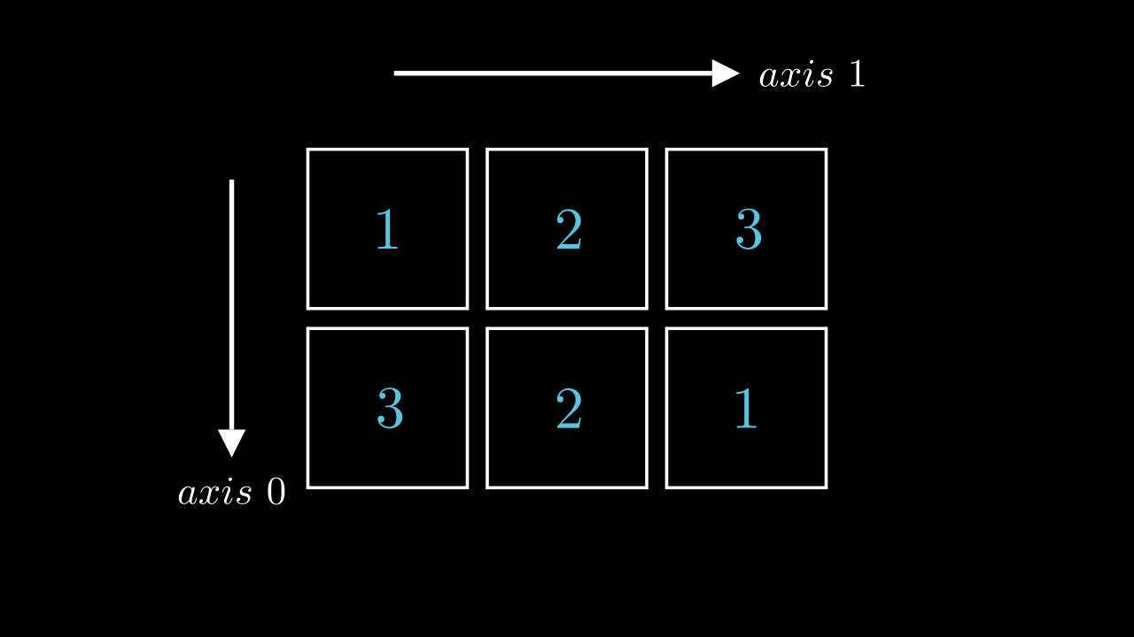
It’s not enough to know how many axes there are, we also must know to which direction they correspond to. As an example let’s imagine an arbitrary 2D matrix. Since it has two dimensions there must be two axes. These dimensions are usually referred to as rows and columns. Naturally, axes are closely related to them. Axis \(0\) corresponds to rows and points in the direction of row increase - downwards, while axis \(1\) corresponds to columns and points in the direction which they increase - to the right.
A question you might ask: “What if we were to add another dimension, in what direction axis \(2\) will point?”. Well, the answer is very intuitive — it will point in the direction of depth’s increase. And if one more? This one is a bit harder to tell. However, it might be useful to remember that since numpy axis are exactly like coordinate system axes it means they form a right-handed coordinate system. Knowing this and direction of axis \(0\) is enough to deduce directions of all other axes.
Working with axes #
Now, let’s look at how two work with axes. There are two common operations that can be performed with axes: indexing and applying numpy operation.
Indexing #
Using axes to index into numpy array is straightforward and is no different from indexing multidimensional arrays in other languages. Again, taking 2D matrix as an example, to choose an element we must specify a row (axis \(0\)) and a column (axis \(1\)). As an example let’s look at this matrix
a = np.array([[1,2,3],[3,2,1]])
print(a)
print("With shape")
print(a.shape)

"""
[[1 2 3]
[3 2 1]]

With shape
(2,3)
"""
and see what’s the element which is in the second row last column
print(a[1][2])

"""
1
"""
Operations #
There are tens on different operations that can be applied to numpy arrays. Most of those operation accept axis as one of its parameters. This is the part that some numpy beginners find confusing.
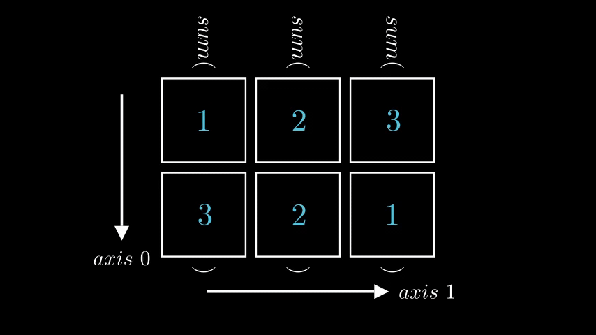
Let’s look at the very common operator sum, an aggregation operator which simply sums elements of a matrix. Let’s look at the 2D matrix from previous example and try to calculate sum of each row.
Usually the thought process goes like this: “I need to calculate sum of each row. When indexing axis \(0\) corresponds to rows, hence i need to call sum with axis=0”
Let’s do exactly that and see what we get!
row_sums = np.sum(a, axis = 0)
print(row_sums)

"""
[4, 4, 4]
"""
Well, this is definitely not what we wanted. Since there are two rows, we expect to get only 2 values, but instead we got 3, which corresponds to number of columns. So, when indexing axis \(0\) corresponds to rows, but when using it with operators it corresponds to columns?
Yes and no.
Let’s forget about aggregated values for a second and see what shape we get when we run sum with different axes as arguments.
print("Shape of original matrix")
print(a.shape)
print("Shape of sum with axis = 0")
print(np.sum(a, axis = 0).shape)
print("Shape of sum with axis = 1")
print(np.sum(a, axis = 1).shape)

"""
Shape of original matrix
(2,3)
Shape of sum with axis = 0
(3,)
Shape of sum with axis = 1
(2,)
"""
We should notice that It seems like we need to pass 1 as axis argument, because with this argument we get two values. Also, it looks as if axis specified by axis argument is collapsed.
This is much closer to the truth.
To get a full picture let’s look at another operation: repeat. It repeats elements of the arrays specified number of times. As sum it accepts axis as one of its parameters. Let’s setup repeat to double number of elements and run it with both axes again focusing on shape and not on the result itself.
print("Shape of original matrix")
print(a.shape)
print("Shape of repeat with axis = 0")
print(np.repeat(a, 2, axis = 0).shape)
print("Shape of repeat with axis = 1")
print(np.repeat(a, 2, axis = 1).shape)

"""
Shape of original matrix
(2,3)
Shape of repeat with axis = 0
(4,3)
Shape of repeat with axis = 1
(2,6)
"""
Look at this! With repeat axis parameter does control what we expect: with axis = 0 there are twice as many rows and with axis = 1 there are twice as many columns. Does it mean that axis corresponds to different notions in sum and repeat?
No!
In both cases axis controls direction along which an operation is applied and behaviours that are different at the first glance is nothing more than an artefact of types of operations: sum contracts and repeat expands matrix. If numpy would have treated dimensions a bit differently, for np.sum(a, axis = 0).shape we would have gotten (1, 3) and for np.sum(a, axis = 1).shape would have been (2, 1). Now there is no discrepancy.
Actually, if we go back to the documentation of sum and repeat and read what axis parameter means we would see in both cases phrase “axis along which” used. It is such an important concept that you even find it in a glossary!
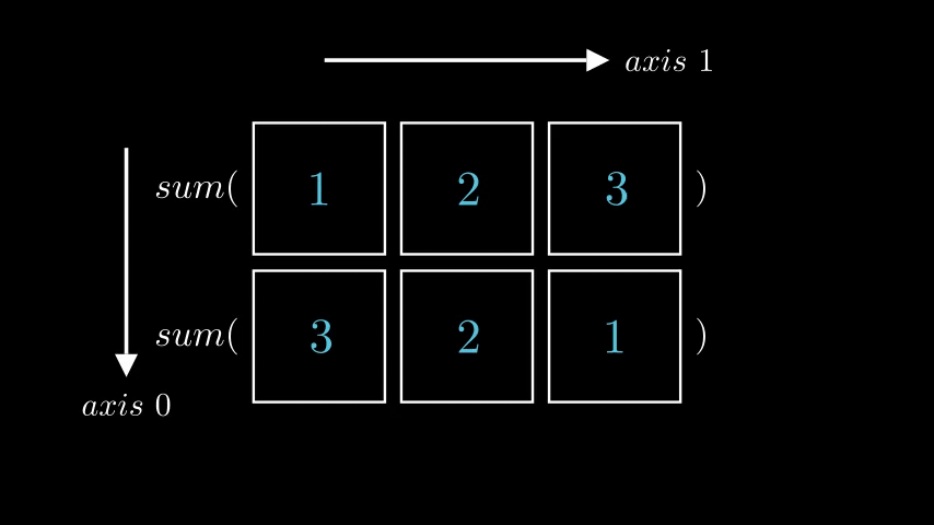
With newfound understanding let’s go back to what we started with: finding a sum of each row. Now we know that the correct axis to use is 1.
row_sums = np.sum(a, axis = 1)
print(row_sums)

"""
[6 6]
"""
which is exactly the correct answer.
And visually it looks like this, where left animation visualizes np.sum(a, axis = 0) and right animation visualizes np.sum(a, axis = 1)
 |
 |
With all that the thing that you need to remember is
axis argument controls axis along which operation is applied
Several axis #
Sometimes axis accepts not only integers (single axis), but also tuples (several axis). Event though there is more than one axes the concept is the same: operation is applied along each axis in the order of axis present in the tuple
Default value #
axis is a named argument which means if you don’t supply a value a default one is gonna be used. For most operation the default value is None which usually (not always) means operation will be applied across all axes. Sometimes this is what you want, but most of the time it is not. Therefore it is important to check what axis argument controls and what default value corresponds to.
TLDR #
Axis is another term for dimension. Axes are referred by numbers, first access being \(0\). Axis \(0\) corresponds to rows — height, axis \(1\) to columns — width, axis \(2\) to depth, etc. When indexing axes behave as expected: axis \(0\) chooses row, axis \(1\) chooses column, etc. When applying operation to numpy array axis controls along which axis operation is applied.